Power BI in itself has a lot of features and functionalities which help you with your job or business. However, Power BI itself won’t solve all your problems which in some cases you may want to peer with other services.

Power BI Premium Capacity

By default, most people will use Power BI pro license level. But when should you consider to leverage Power BI premium capacity? There are couple of things you may need to consider: 1. to store larger datasets, 2. Allow faster DirectQuery /Live Connection query, 3. Support Paginated Reports, 4. Allow unlimited Content Sharing for both internal or external viewers.

If you want to know more information about Power BI Premium Service, please refer to this Microsoft doc.

Azure Synapse Analytics

Azure Synapse Analytics (ASA) is a great alternative for your Power BI model Development. It allow you to query petabytes of data in a performant way with reasonable price by leveraging Direct Query mode of Power BI. ASA Data Pool is a MPP(Massive parallel processing) solution with the Result Set Catches and Materialized View built in so that it enabled high volumes of concurrency quires. Build your data warehouse in ASA as compare to Power BI you can provide Enterprise-grade data preparation and data warehousing solution which allows single source of trues for Power BI and other application and centralized security. In addition, the studio experience within ASA allow team collaboration amongst (data scientists, data engineers, DBA, and BI Developers).

For more information about this topic, please refer to this whitepaper.

AI and Machine Learning Services

There are 3 ways you can extend your BI data to AI insights within Power BI.

1. Auto ML in Power BI Dataflow; Official Doc Tutorial

2. Calling Existing Cognitive Services; Official Doc Tutorial

3. Call Machine Learning Models which Stored in Azure Machine Learning Services. Official Doc Tutorial

Azure Data Lake Storage Gen 2

By default, data used with Power BI is stored in internal storage provided by Power BI. With the integration of dataflows and Azure Data Lake Storage Gen2 (ADLS Gen2), you can store your dataflows in your organization’s Azure Data Lake Storage Gen2 account.

Simple put, Dataflow within power bi is Power Query + Common Data Model (CDM). With the Common Data Model (CDM), organizations can use a data format that provides semantic consistency across applications and deployments. And with Azure Data Lake Storage gen2 (ADLS Gen2), fine-grained access and authorization control can be applied to data lakes in Azure.

For more information about this topic, please refer to this official doc.

Azure Analysis Service

The core data modeling part of Power BI is actually Analysis Services. So using Azure Analysis Services (AAS), you can create data models independently from Power BI services. Right now the largest SKU of AAS allows you to store up to 400GB of data. You can allow different report applications (like Power BI, Tableau, Excel) to connect to your AAS models. Within Microsoft, The Analysis Services team is a sub team of Power BI. The product roadmap for Power BI is to minimize the data modeling experience between Power BI premium capacity and Azure Analysis services. That’s why are are seeing the recent updates from Power BI included those enterprise grade data modeling capability such as increased dataset limited, XMLA endpoint, and workflow pipeline, etc. However, most of those features are in preview and is about to go GA. In short, if you are migrating from your on premise SSAS model to Azure or you do not want to wait for the PBI features go to GA, then AAS is your easiest option. Otherwise, choose Power BI premium to host your reports and data models is strongly recommended.

Reference: https://azure.microsoft.com/en-us/services/analysis-services/#overview

Power Automate & Power App

When I think about Power BI with other Power Platform tools, I think it is a Insights + Action Play. You can use Power BI to get insights from your data and then use Power Automate or Power App to take action out of it.

The Bi-Directional Connectors allow you to connect the services between each other which means you can embed power bi report to power app and you can embed power app to power bi.

Reference:

1. https://docs.microsoft.com/en-us/power-bi/collaborate-share/service-flow-integration

2. https://powerbi.microsoft.com/en-us/blog/power-bi-tile-in-powerapps

Azure Logic Apps, Azure Monitor log analytics

•Synchronously Refreshing a Power BI Dataset using Azure Logic Apps.

Reference: A Step by Step Community Blog Post.

•Use Power BI to understand your Logic Apps Consumption Data

Reference: A Microsoft Blog

•Use Azure Monitor Logs you can understand your Power BI embedded consumption. You can also use Power BI to create customized report out of your Azure Monitor Logs.

Reference: Microsoft Doc

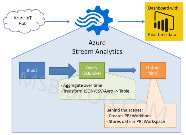
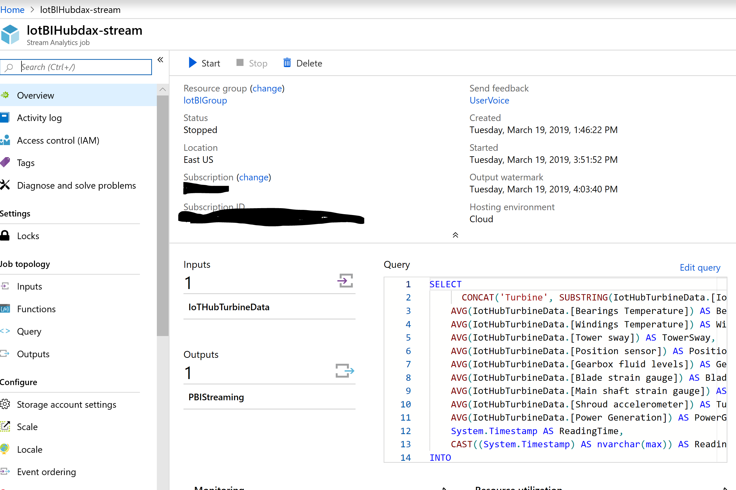
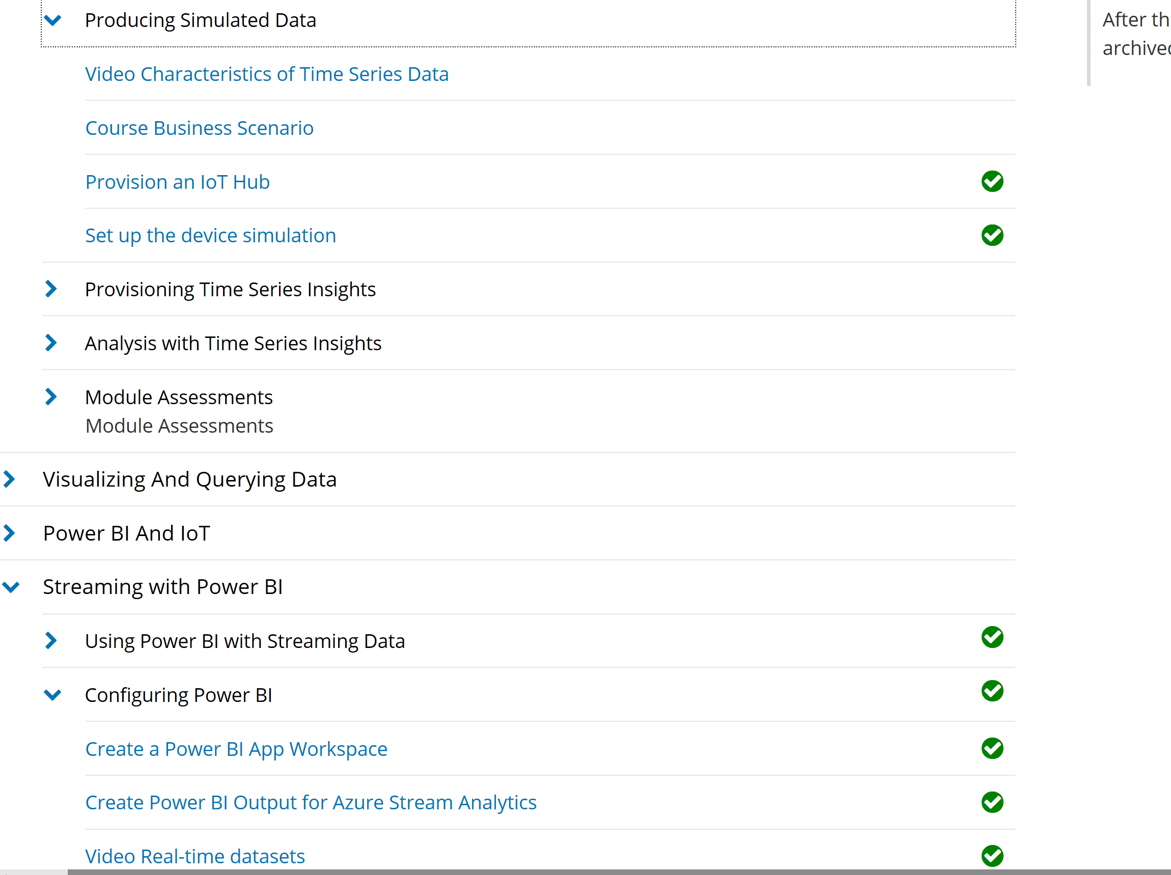
Azure Streaming Analytics

This is a solution for true real time analytics in Power BI. It enables you to visualize your IOT or Events data.

Typical Architectural is Device Data -> Event Hub -> Azure Streaming Analytics -> Power BI Streaming Datasets -> Power BI Dashboards.

Reference: Official Document

My blog: https://xuanalytics.com/2019/03/24/simulated-streaming-data-power-bi-embedded/

Microsoft Teams

You can Add your Power BI report as an App to Teams.

Reference: Official Doc

Also if you have admin credentials to Teams, then you can Analyze Call Quality Data in Power BI.

Reference: Official Doc

Dynamics 365

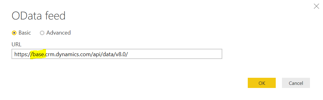
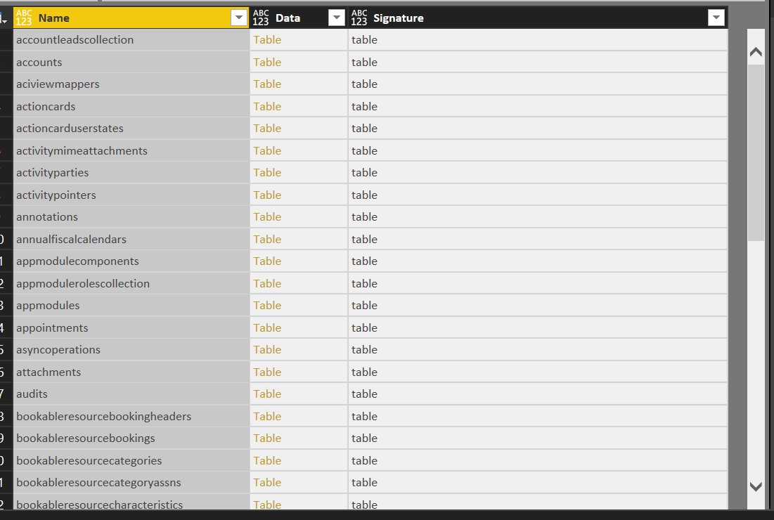
•You can use Power BI to analyze the data in Dynamics 365 (OData or Entity Store from LCS)

•You can Pin your Power BI visuals to Dynamics 365

•You can use existing PowerBI.com solutions from Lifecycle Service

•There is a Power BI Embedded Experience within Dynamics (Boxed)

References:

1. Official Doc Configure Dynamics 365 Power BI Integration
2. Official Doc: PowerBI.com Service in Dynamics F&O
3. Official Doc: Get Dynamics Data in Power BI using Business Central
4. Official Doc: Customize Dynamics F&O analytical workspace

In summary, there many other services inside or outside Microsoft products portfolio works will with Power BI. So consider think outside of the box and create different solutions for your business.

Your friend,

Annie

This post is about something new I have tried last week. The goal was to create simulated streaming data source, feed it into Power BI as a streaming dataset, create a report out of the streaming dataset, and then embed it to an web application. With proper directions provided by my teammates, I finished the implementation from end to end within 1.5 hours. I was super impressed by how awesome it is and how easy it is to implement so that I want to share those directions to you.

Main Step 1 Create simulated streaming data and push it to a Power BI as streaming dataset

1. The basic steps include:
   1. Set up an Azure IOT hub to capture the data
   2. Use IOT Simulator https://www.azureiotsolutions.com/Accelerators#dashboard to simulate streaming data
   3. Create a Power BI App Workspace in PowerBI.com
   4. Set up Streaming Analytics Job to connect data coming from IOT hub to Power BI dataset

2. There is a free tutorial course from EDX talks about the above steps in details. You do not have to finish all the tutorial and you can just go through the ones in green check marks as shown in below.

https://www.edx.org/course/iot-business-intelligence-for-iot-solutions

                 

Main Step 2: Create a Power BI report using the streaming dataset

1. Open Power BI Desktop
2. Click on Get Data
3. Choose ‘Power BI dataset’
4. Choose the Power BI streaming dataset you just created from Main Step 1

5. Once you connected to the streaming dataset, you can use it to create your graphs and charts.
6. Lastly, click ‘Publish’ to save your PBIX file back to PowerBI.com.

Main Step 3 Embed your Power BI report to your application

1. If you need to embed your report into your application, please follow this tutorial https://docs.microsoft.com/en-us/power-bi/developer/embed-sample-for-customers

This tutorial introduced the following important topics which we have not done in the previous steps

1. How to register an application in Azure Active Directory (Azure AD) which allows your application to interact with Power BI.
2. It provides a sample application package from GitHub. You can just update webconfig file of the sample package on applicationID you just created, the workspaceid where your report locates, the reportid of your report, and your Power BI credential.

4. Lastly, to set up automatic refresh of your streaming dataset on your application, please try the following blog

http://radacad.com/integrate-power-bi-into-your-application-part-4-refresh-data-set

 

Thank you,

Your friend, Annie

 

I finished my Fundamental Finance Accounting course last week. I learned 2 awesome functions which helps which which projects to undertaken. Frist is NPV net present value and the second is IRR(Internal Rate of Return). I found those two are so powerful to use helping to decide which investment to choice so I want to implement in DAX. Fortunately, in DAX there are two functions XNPV and XIRR which I can choose to use. I found that XNPV and XIRR are also in excel and would be a replacement of IRR and NPV.  They have slightly different calculation details but the purpose are the same. You can find http://www.differencebetween.net/business/finance-business-2/difference-between-npv-and-xnpv/ and https://corporatefinanceinstitute.com/resources/knowledge/modeling/xirr-vs-irr-excel-financial-model/  for more details.

The Excel XNPV function is a financial function that calculates the net present value (NPV) of an investment using a discount rate and a series of cash flows that occur at irregular intervals. Calculate net present value for irregular cash flows. Net present value. =XNPV (rate, values, dates)

The Excek XIRR(Internal Rate of Return) is the discount rate which sets the Net Present Value (XNPV) of all future cash flow of an investment to zero.  If the NPV of an investment is zero it doesn’t mean it’s a good or bad investment, it just means you will earn the IRR (discount rate) as your rate of return. =XIRR(values,dates,guess)

The challenge in DAX, I found, is that , we may not have the date field. For example, we may just calculate a intial investiment and an estimate assuming paying amount every year or every month in the future. Something like this:

So in DAX, we can create table variable in the Measure to leverage XIRR and XNVP.

XIRR =
VAR cashflowtable =
    UNION (
        GENERATE (
            GENERATESERIES ( YEAR ( NOW () ), YEAR ( NOW () ) ),
            VAR inc = [Value]
            RETURN
                ROW (
                    "date", DATE ( inc, 1, 1 ),
                    "Values", SUM ( 'Considered Project'[Initial Inventestment] )
                )
        ),
        GENERATE (
            GENERATESERIES ( YEAR ( NOW () ) + 1, YEAR ( NOW () ) + [Investment Years] ),
            VAR inc = [Value]
            RETURN
                ROW (
                    "date", DATE ( inc, 1, 1 ),
                    "Values", SUM ( 'Considered Project'[Annual Cash flow] )
                )
        ),
        GENERATE (
            GENERATESERIES (
                YEAR ( NOW () ) + [Investment Years],
                YEAR ( NOW () ) + [Investment Years]
            ),
            VAR inc = [Value]
            RETURN
                ROW (
                    "date", DATE ( inc, 1, 1 ),
                    "Values", SUM ( 'Considered Project'[Exit Value] )
                )
        )
    )
RETURN
    XIRR ( cashflowtable, [Values], [date] )

XNVP =
VAR cashflowtable =
UNION (
GENERATE (
GENERATESERIES ( YEAR ( NOW () ), YEAR ( NOW () ) ),
VAR inc = [Value]
RETURN
ROW (
"date", DATE ( inc, 1, 1 ),
"Values", SUM ( 'Considered Project'[Initial Inventestment] )
)
),
GENERATE (
GENERATESERIES ( YEAR ( NOW () ) + 1, YEAR ( NOW () ) + [Investment Years] ),
VAR inc = [Value]
RETURN
ROW (
"date", DATE ( inc, 1, 1 ),
"Values", SUM ( 'Considered Project'[Annual Cash flow] )
)
),
GENERATE (
GENERATESERIES (
YEAR ( NOW () ) + [Investment Years],
YEAR ( NOW () ) + [Investment Years]
),
VAR inc = [Value]
RETURN
ROW (
"date", DATE ( inc, 1, 1 ),
"Values", SUM ( 'Considered Project'[Exit Value] )
)
)
)
RETURN
XNPV ( cashflowtable, [Values], [date], [Interest Rate] )

Hopefully, you find this helpful.

Thanks,

your friend, Annie

Within Microsoft lastest PowerBI update, the one exites me most is that we can link PowerBI data flow to Azure data lake storage account.

Benefits are:

1. When you have a PBIX imported mode reaching more than 1 GB and you are not Primier memeber you can not publish to PowerBI.com. However, with DataFlow in PowerBi you can save upto 10 GB data.
2. Your workspace members are able to reuse the same data flow as souce of their PowerBI file.
3. When liked to Azure Data Lake Sotrage Gen 2 you can use data got from PowerBI Dataflows as data source across your Azure applications.

To try this, you need to have the following things

You have PowerBI-Pro license and above.

You are an admin to your Azure portal. (Or you are good friend of your admin ^_^)

There are few things I found out when I did my experiment and I think you might face are:

1. You can use blank query to copy M Codes from your Power Queries
2. If you have a table function to transfer and you don’t have primier account, you can still do so by select “do not load”
3. To configure Azure Data Lake Gen 2 connect to PowerBI, follow this document from microsoft. https://docs.microsoft.com/en-us/power-bi/service-dataflows-connect-azure-data-lake-storage-gen2
4. When you configured everything right according to the above microsoft document. You may still have issue like I did. Please follow the following communication string  to see the lastest udpate on the PowerBI community discussing. https://community.powerbi.com/t5/Service/Power-BI-Dataflow-to-Azure-Data-Lake-Gen2-Setup/td-p/583564

Latest update, Microsoft team has fixed the above. Now I have tested and works fine.

Thanks,

Your friend, Annie

Recently, I need to do a data warehouse migration for a client. Since there might be some difference between the Dev environment source databases and Prod environment source databases. The migrated SSIS packages for building data warehouse might have some failures because of the changes. So the challenge is how can I validate all my DW packages (100 +) all at once.

There are a good amount of posts out there to do one package validation at a time using the Management Studio GUI (just right click on the package under SSIS Catalog)

Or using T-SQL store procedure [SSISDB].[catalog].[validate_package]. Here is the explanation of this store procedure from Microsoft.

To get the validation all at once, we can use a loop query to execute [SSISDB].[catalog].[validate_package] one by one.

Here is the code I created and would love to share.

Couple days ago, a client of mine is asking me to build a Dynamics CRM Online user activities dashboard. In Dynamics CRM On-premises version, I know, this information resides in audit table. However, with Dynamics CRM online, I am not able to access directly to the backend database. Fortunately, there are few PowerBI content packs for Dynamics CRM online out there in market place so that I was able to read through the PBIX file and find out how PowerBI is connected to the Dynamics CRM Online data.

PowerBI is using OData as data source to connect to Dynamics CRM online web services which gives you almost all data available (There are still some important fields and tables which are in On-premises version and causing the challenge of build reports effectively) . You just need to change the highlighted piece below to your organization CRM web name.

 

I did find the ‘Audit’ table available. However, there are few challenges to interpret the data. I am listing the challenges below and the steps I handled it.

1. Initially, the ‘Audit’ table is blank.
   • This is because in CRM online you need to enable the setting of Audit Tracking. You can follow this blog to enable it.
2. Every field is in its code or id format. And, there is no mapping table in Odata connection to map between field id and field value.
   • I have check the Microsoft provided content pack and found out those mapping table are hard coded. So I have to google the CRM Audit Entity documentation in Microsoft to get the hard coded mapping for the following fields.
     • Operation – The action that causes the audit – It will be create, delete, or update
     • Action – Actions the user can perform that cause a change
     • 
3. You can expand the userID field to get the information  (such as full name, login account, address, etc.) of user who caused a change. This however, only provide information for users who make changes like ‘create’, ‘update’, and ‘delete’. For ‘access’ status, this userid only reflect as ‘SYSTEM’ as the user.
   • To get the information about the user’s name who access CRM, we need to link the ‘_objectid_value’ field from Audit table to the ‘UserId’ field from systemusers table.
4. Missing ‘ObjectTypeCode‘ field. This is the key field is missing from this table for the Odata connection data pull. Thus, we are not able to find which entities the changes were made on.
   • Unfortunately, I have not find a solution for this unless CRM team reveal this field for the CRM Audit Entity.
   • If this field is available in the future, we can use this field in combine with ‘Attributemask’ fields to get the column names of the objects which has been changed. So that we can build further analysis report.

For now, with the information we can get, we can start to build dashboard with user login activities.

Thanks.

I love that you can always find multiple ways to solve one problem. Inspired by the Youtube video by Guys in the cube and blog reading from SQLBI.com, I found there are two ways to dynamically change measures in the same visual. The first way is more towards front end report developer using bookmark and the second way is more towards data modeler using a technique called disconnected tables.

Bookmarks method:

The basic steps are:

1. Enable Bookmarks under File ->’Options and Settings’ ->Options->Preview Features->’Bookmarks’
2. Create one visual for example a bar chart with first measure, for example Revenue by Sales Territory
3. and copy paste the visual 2 times. in the coped visuals replace the measure you want to replace. For example cost by sales territory.
4. Overlay the three visuals together.
5. Go to ‘View’ on the top tool panel and make sure ‘Bookmarks Pane’ and and ‘Selection Pane’ are checked
6. Add bookmarks with selection of visuals to be visible associated with the bookmark you created
7. .
8. Add the images/shapes which represent the measure you want to select on and link it to the bookmark you created.
9. 

Disconnected Table method:

This method is more towards PowerBI modelers. Basically, the idea is to have a Field in a independent table (no relationship to other tables) as Slicer with your measure choice and then create a measure using SELECTEDVALUE function to have the measure dynamically switch referring measures based on the choice made on the slicer.

Step 1. Created an new table called ‘Measurechoice’ like image below.

Step 2. Create a measure called ‘Selected Value’

Selected Value = SWITCH(SELECTEDVALUE(‘Measurechoice'[Index]),1,[Total Revenue],2,[Total Cost],3,[Total Profit],BLANK())

Step 3. Create a slicer using ‘MeasureChoice’ from the new table created.

Step 4. Create a visual use the ‘Selected Value’ as Value

Personally, I like the disconnected table method because I don’t need to spend time on creating images and link bookmarks. However, the bookmarks choice can help dynamically change the title of the visual and give you the ability to change the layout of your bookmark views. Now it is your choice to choose either one to fit your reporting needs.

Thanks for spending time reading this blog.