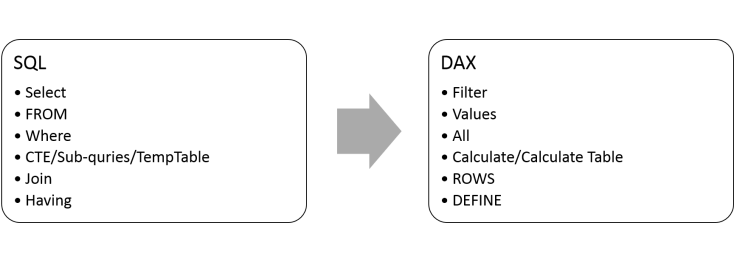
New DAX Functions only in SSAS 2016 and Above

SQL Server 2016 Analysis Services (SSAS)*, Power Pivot in Excel 2016, and Power BI Desktop include the following new Data Analysis Expressions (DAX) functions:

Date and Time Functions

CALENDAR Function
CALENDARAUTO Function
DATEDIFF Function

Information Functions

ISEMPTY Function
ISONORAFTER Function

Filter Functions

ADDMISSINGITEMS Function
SUBSTITUTEWITHINDEX Function

Math and Trig Functions

ACOS Function
ACOSH Function
ASIN Function
ASINH Function
ATAN Function
ATANH Function
COMBIN Function
COMBINA Function
COS Function
COSH Function
DEGREES Function
EVEN Function
EXP Function
GCD Function
ISO.CEILING Function
LCM Function
MROUND Function
ODD Function
PI Function
PRODUCT Function
PRODUCTX Function
QUOTIENT Function
RADIANS Function
SIN Function
SINH Function
SQRTPI Function
TAN Function
TANH Function

Statistical Functions

BETA.DIST Function
BETA.INV Function
CHISQ.INV Function
CHISQ.INV.RT Function
CONFIDENCE.NORM Function
CONFIDENCE.T Function
EXPON.DIST Function
GEOMEAN Function
GEOMEANX Function
MEDIAN Function
MEDIANX Function
PERCENTILE.EXC Function
PERCENTILE.INC Function
PERCENTILEX.EXC Function
PERCENTILEX.INC Function
SELECTCOLUMNS Function
XIRR Function
XNPV Function

Text Functions

CONCATENATEX Function

Other Functions

GROUPBY Function
INTERSECT Function
NATURALINNERJOIN Function
NATURALLEFTOUTERJOIN Function
SUMMARIZECOLUMNS Function
UNION Function
VAR

How to create customized color themes for your PowerBI visuals

I found it is just as important to have a nice looking dashboard/reports as the data itself. In this blog, I want to share with you some good tricks which I learned recetly from PowerBI.com and a Youtube channel EnterpriseDNA to create customized color themes in PowerBI desktop.

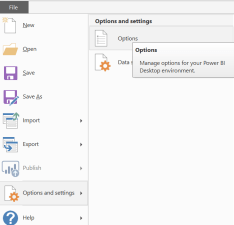
By default, the customized theme feature is not enabled in PowerBI desktop. So what you need to do is go to ‘File’ -> ‘Options and Settings’

PowerBI Option Change

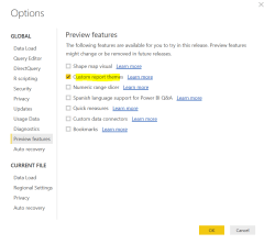
then, enable the ‘Custom Report Themes’ in ‘Preview Features’ section.

Custom Report Theme Enable

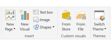
After restarting your PowerBI desktop, you will see ‘Themes’ under ‘Home’ tab

Themes tab

By choosing ‘Switch Themes’, you can import your customized theme saved as JSON file.

Typical JSON Code for themes like this

{    “name”: “St Patricks Day”,
“dataColors”: [“#568410”, “#3A6108”, “#70A322”, “#915203”, “#D79A12”, “#bb7711”, “#114400”, “#aacc66”],
“background”:”#FFFFFF”,
“foreground”: “#3A6108”,
“tableAccent”: “#568410” }
From <https://powerbi.microsoft.com/en-us/documentation/powerbi-desktop-report-themes/>

But, how could we get a good color combination which looks good if I am not a artist?

Usually, I will create the foundation colors based on company logo or image. Since Halloween is coming soon, let’s use a Halloween picture as an example.

There is a site recommended http://palettefx.com/ which helps you to find all the colors used in the image.

Color Pickers

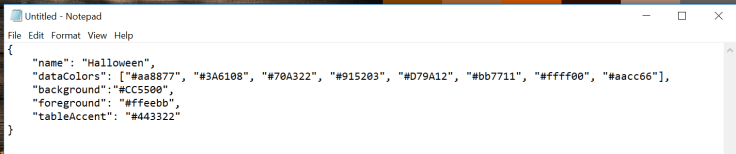
After that, you use Notepad and edit the JSON code I shared above and save as .json file. Json code

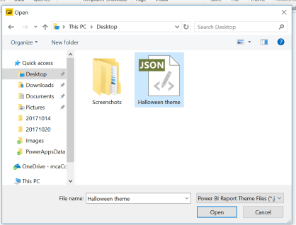
Now, you can import the JSON file into PowerBI use the ‘Switch Themes’ add-in we got as your customized theme.

Jason file

Now, you can use your new customized theme to build your PowerBI reports!

There is a PowerBI theme Gallery: https://community.powerbi.com/t5/Themes-Gallery/bd-p/ThemesGalleryHopefully it helps.

Your friend, Annie


From SQL to DAX- ‘Lead’ and ‘Lag’ window functions

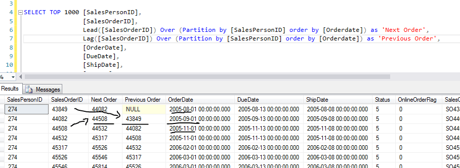
In SQL, we have two window functions call lead and lag, and with these two functions, you can get the previous and next value of a column partition by and order by other columns in a table.

Use our Advanturework Sales.SalesOrderhead table as an example. The following code can give you the previous and next SalesOrderID for a SalesPersion order by OrderDate.Lead and Lag SQL code

However, it is a very expensive function because the SQL engine need to fetch through the entire table for every row calculation where the functions are called.

It is much faster to use DAX in SSAS tabular model in this case, where the column-store and vertipaq compression technologies are embedded. To use DAX replace lead and lag function, we will be using a key function in DAX called ‘Earlier’.

Using the same example mentioned above,

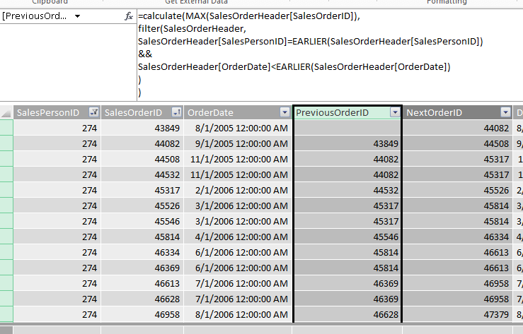
You can write Previous Order ID calculate column like this:DAX previous and next.PNG

As we know, ‘Calculate’ Function covers the current row context to filter context of the calculation (as the first argument) inside ‘Calculate’. However, the filter contexts (second and the following arguments of ‘Calculate’) created in side ‘Calculate’ block those external filter contexts when they are referring the same columns. In this case, ‘Filter’ function blocked all the filter contexts added externally on the ‘SalesOrderHeader’ table, in other word, the calculation in the first argument of ‘Calculate’ MAX(SalesOrderHeader[SalesOrderID]) don’t know which row it is at SalesOrderHeader table. Only the ‘Earlier’ function brings the previous filter contexts back, which allows MAX(SalesOrderHeader[SalesOrderID]) aware of which row it is at.

Using the second row of the above screenshot as an example, the DAX calculation of PreviousOrderID column can be explained as:

Find the max SalesOrderID where SalesPersonID equal to the SalesPersionID of existing row (called by ‘Earlier’ function) which is ‘274’ and OrderDate are older than the OrderDate of existing row (called by ‘Earlier’ function) which are all the records with OrderDate older than 9/1/2015. Thus, the result is ‘43846’.


Thanks.

Your friend Annie.


How to use Dynamic Management Views against on your Desktop PowerBI reports

Power BI contains a local instance of Analysis Services tabular model. By querying Dynamic Management Views (DMVs) query against PowerBI desktop, we can get metadata information about your PowerBI model.

Here are the steps to do so:

Step 1: Open your Power BI report

Step 2: Find your Power BI Analysis Model Instance Port ID.

There are two ways to do that:

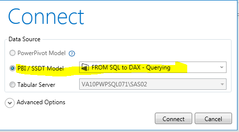
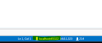
Option 1: Open up DAXStudio (a great free tool to help you develop DAX). And then connect to the Power BI report you opened.

Get DAX 1.PNG

Then, Find the local Analysis Service instance address of this Power BI report on the right bottom of the DAX studio window

Get DAX 2.PNG

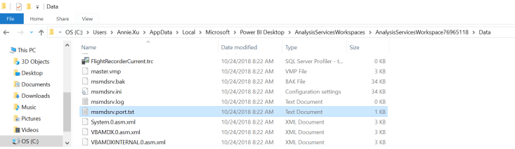
Option 2: Fine the Power BI temp directory
C:\Users\username\AppData\Local\Microsoft\Power BI Desktop SSRS\AnalysisServicesWorkspaces\…\Data

PowerBI Port


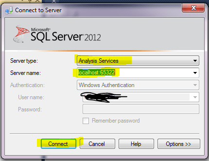
Step 3. Open SQL Server Management Studio. And connect to the local instance of Analysis

Get DAX 3


Step 4: Create an new query against the only Database under the local instance

Get DAX 4

Step 5: In the query window, you can then run the Dynamic Management Views (DMVs) to Monitor your PowerBI local instance.

The ones I use often including the following:

  • The DMV provide the DAX query behind the report:
Select * from $System.discover_sessions
  • This DMV Provide you all the fields in your model
Select  * from $system.MDSchema_hierarchies
  • This DMV Provide you all the measures in your model
Select * from $System.MDSCHEMA_MEASURES

Find relationships:

Select [ID], [ModelID], [IsActive], [Type], [CrossfilteringBehavior], [FromTableID], [FromColumnID], [FromCardinality], [ToTableID], [ToColumnID], [ToCardinality], [ModifiedTime]
from $SYSTEM.TMSCHEMA_RELATIONSHIPS
Select [ID], [ModelID], [Name]from $SYSTEM.TMSCHEMA_TABLES
Select [ID], [TableID], [ExplicitName] from $SYSTEM.TMSCHEMA_COLUMNS

For More DMV, there is a good post: https://datasavvy.me/2016/10/04/documenting-your-tabular-or-power-bi-model/

Bonus

If you do not have SSMS, you can use Power Query in Excel or Power BI to query those DMVs, here is an sample M query.

let
    Source = AnalysisServices.Database(TabularInstanceName, TabularDBName, [Query=”Select [ID], [TableID], [Name], [Description], [DataSourceID], [QueryDefinition], [Type], [Mode], ModifiedTime from $SYSTEM.TMSCHEMA_PARTITIONS”]),
    #”Renamed Columns” = Table.RenameColumns(Source,{{“ID”, “ID”}, {“DataSourceID”, “Data Source ID”}, {“QueryDefinition”, “Query Definition”}, {“ModifiedTime”, “Modified Time”}})
in
    #”Renamed Columns”

Thanks

Your friend, Annie


Compare Formula Engine VS. Storage Engine in SSAS Tabular

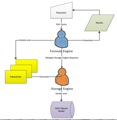
To improve SSAS tabular performance or to improve your DAX query, it is important to know the different between formula engine and storage engine. Here, I have created a table for you to better distinguish these two in Tabular (I need to reinforce it is for tabular modeling not multidimensional because the back end technology used is quite different). Both engines play vital roles to process DAX query requests.

FE and SE

Category Formula Engine Storage Engine
Query received Interpret DAX/MDX formula Can handle single logic (xmSQL) from formula Engine
Target Data Iterate over datacaches produced by storage engine (datacaches are in-memory tables) Iterate over compressed data in vertipaq column stores
Result Produce result set and send back to requestor Produce Datacaches send back to formula Engine
Thread Single – Threaded Multi – Threaded
Cache utilization No Yes
Area of focus for  Performance Tuning Check physical plan for bottleneck Check xmSQL query for bottleneck


DAX – Filter Context V.S Row Context

A key to understanding DAX is to distinguish Filter Context and Row Context.

Here are definitions of each context.

Filter Context: can be simply defines as filter context the set of filters applied to the evaluation of a DAX expression, usually a measure, regardless of how they have been generated. Usually, every cell of a report has a different filter context, which can be defined implicitly by the user interface (such as the pivot table in Excel), or explicitly by some DAX expression using CALCULATE or CALCULATETABLE. Filter Context always exist before a DAX expression been evaluated.


Row Context: the concept of row context is always exist in a DAX expression. In order to get the value of a DAX expression, you need a way to tell DAX the row to use AKA checking the current row of a table and provide the value back. You have a row context whenever you iterate a table, either explicitly (using an iterator) or implicitly (in a calculated column).


Use one DAX measure as an Example:

SumofProductSalesAmount:=SUMX(

VALUES([Product].[ProductName]),   

CALCULATE (

        [Sales Amount]

    )

)


Explain in detail of this calculation:

  1. VALUES Function returns a table, meaning it provide All the Distinctive ProductName back as a table outcome
  2. SUMX iterate each row of the table in its first argument, then it aggregate the value each row returns in sum. In this case, for each row of a table which provided by VALUES function AKA for each product, it calculate the value in the second argument of the SUMX function. Then, Sum all the value together and return back to the caller.
  3. Things happens outside CALCULATE Function are all treated as Filter Context of the CALCULATE expression. In this case, there are two places feeding the CACULATE section with Filter Context.
    • First place is, the Current Row defined by SUMX, in our case, it is the Current Row of VALUES([Product].[ProductName]) which will be a specific Product depends on where the iterator at. Meaning Evaluated [Sales Amount] Measure with a filter which limit to a certain Product, and then provide the value (sales amount) back.
    • Second Place is, whenever this measure [SumofProductSalesAmount] exposed in a cell user application (like Excel, PowerBI, SSRS), it exposed in a filter context set on that specific Cell. Depends on wherever your cell is at you have different filter context. For example you may have a filter on a cell to limit the time frame to 2017, etc.


Thanks,

Your friend – Annie.

Situations to use Multidimensional SSAS model over Tabular Model

4154_tabular_vs_multidimensional

I was introduced with SSAS modeling about 5 years ago. At that time, our team is recommended by Microsoft to use their new modeling technology called Tabular SSAS modeling. Since then, our team started to build multiple tabular models, and those models are growing larger and larger with more complicated calculations. We love tabular modeling because it uses xVelocity engines (Vertipaq – in memory analytic engine and memory optimized ColumnStore index) which means it is super fast because of the in memory storage and it is mulch easier to implement because it uses relational modeling structure which we are familiar with, the script language DAX is kind of like Excel formula to start, and we don’t need to consider set, MDX calculations, aggregations, and storage modes etc. which makes Multidimensional Modeling very complex and difficult to learn.

However, with more complicated requirements come in, we are facing some challenges with current Tabular modeling solution.

As of recently, I started to prepare Microsoft BI certification and started to look into Multidimensional modeling. I found out that we may be able to leverage some of its capabilities which already exists in multidimensional modeling which has been exist so many years. I listed some of those capabilities which are not exist in Tabular model yet.

  1. Remote Partitioning (partition can locate in other server)
  2. Multiple Storage mode selection (MOLAP to ROLAP)
  3. Write Back option – customer can write back to the model – only for aggregate function other than Sum (create “what-if analysis”
  4. Aggregations – pre-calculated (can change setting of how much to pre aggregated) need to consider the storage and maintenance required
  5. Many to many relationships
  6. Role play dimensions
  7. Customized Drill-through and other actions (for older version of Tabular we can use BIDS helper to do it. But, for tabular in SQL server 2016 version, it is disabled)
  8. Merge Partitions, ssms will automatically remove but the visual studio workspace project need to update manually.
  9. Calculation Template
  10. Build in Business Intelligent
  11. Process Index (build or rebuild)
  12. Partition Slice – know only pull the model slice information and provide fast finding of the right partition to use to calculate

Thanks,

Your Friend, Annie


Simple MDX Queries

— Single axis

select [Measures].[Sales Amount] on Columns

from [InternetSales];

— Double axis

Select [Measures].[Sales Amount] on Columns,

[Dim Date].[Calendar Year].[Calendar Year].ALLMEMBERS on rows

from [InternetSales];

–two aggregation wrong no supported

Select [Measures].[Sales Amount] on 0,

[Dim Employee].[Reports To].[Level 02].ALLMEMBERS on 1,

[Ship Date].[Calendar Year].[Calendar Year].ALLMEMBERS on 2

from [InternetSales];

–two aggregation right

Select [Measures].[Sales Amount] on 0,

[Dim Sales Territory].[Sales Territory Country].[Sales Territory Country]*[Ship Date].[Calendar Year].[Calendar Year].ALLMEMBERS on 1

from [InternetSales];

–Filter out emplty

Select [Measures].[Sales Amount] on 0,

NON EMPTY ([Dim Sales Territory].[Sales Territory Country].[Sales Territory Country].ALLMEMBERS) on 1

from [InternetSales];

–“ALLMEMBER”

Select [Measures].[Sales Amount] on 0,

NON EMPTY ([Dim Sales Territory].[Sales Territory Country].[Sales Territory Country].ALLMEMBERS) on 1

from [InternetSales];

Select [Measures].[Sales Amount] on 0,

NON EMPTY ([Dim Sales Territory].[Sales Territory Country].[Sales Territory Country].&[Canada]) on 1

from [InternetSales];

–using tuples

Select NON EMPTY [Measures].[Sales Amount] on Columns,

NON EMPTY [Order Date].[Calendar Year].[Calendar Year] on rows

from [InternetSales];

Select NON EMPTY ( [Measures].[Sales Amount],[Order Date].[Calendar Year].[Calendar Year]) on columns

FROM [InternetSales];

–creating a tuple set

Select NON EMPTY {([Measures].[Sales Amount],[Order Date].[Calendar Year].[Calendar Year].&[2006]),

([Measures].[Sales Amount],[Order Date].[Calendar Year].[Calendar Year].&[2007]),

([Measures].[Sales Amount],[Order Date].[Calendar Year].[Calendar Year].&[2008])

} on columns

FROM [InternetSales];

–Multiple Tuple Sets

Select [Measures].[Sales Amount] on Columns,

NONEMPTY(

([Dim Product].[Model Name].Allmembers, {[Order Date].[Calendar Year].[Calendar Year].&[2007]

,[Order Date].[Calendar Year].[Calendar Year].&[2008]}),[Measures].[Sales Amount]

) on rows

FROM [InternetSales];

–Functions

–TOP Percent

Select [Measures].[Sales Amount] on COLUMNS,

TopPercent([Dim Product].[Model Name].[Model Name],50,[Measures].[Sales Amount]) on ROWS

from [InternetSales];

–Top Sum (running total of category aggregattion exceed a certain amount)

Select [Measures].[Sales Amount] on COLUMNS,

TopSum([Dim Product].[Model Name].[Model Name],150000,[Measures].[Sales Amount]) on ROWS

from [InternetSales];

–use set functions

–Members and Allmembers (to see or not to see calculated members)

Select [Measures].[Sales Amount] on COLUMNS,

[Dim Product].[Model Name].[Model Name].Members on ROWS

from [InternetSales];

–non emplty

Select [Measures].[Sales Amount] on COLUMNS,

Non empty [Dim Product].[Model Name].[Model Name].Members on ROWS

from [InternetSales];

–nonemplty function against tuple

Select [Measures].[Sales Amount] on COLUMNS,

Nonempty( [Dim Product].[Model Name].[Model Name].Members, [Measures].[Sales Amount]

) on ROWS

from [InternetSales];

–Top/Bottom Count

Select [Measures].[Sales Amount] on COLUMNS,

TopCount( [Dim Product].[Model Name].[Model Name].Members, 5,[Measures].[Sales Amount]

) on ROWS

from [InternetSales];

Select [Measures].[Sales Amount] on COLUMNS,

BottomCount([Dim Product].[Model Name].[Model Name].Members, 31,[Measures].[Sales Amount]

) on ROWS

from [InternetSales];

— Specifying Axis

Select [Measures].[Sales Amount] on Columns,

[Dim Date].[Calendar Year].[Calendar Year].ALLMEMBERS on rows

from [InternetSales];

–Not supported in SSMS

Select [Measures].[Sales Amount] on 0,

[Measures].[Discount Amount] on 1,

[Dim Date].[Calendar Year].[Calendar Year].ALLMEMBERS on 2

from [InternetSales];

–use tuples instead has to start at 0

Select non empty {[Measures].[Sales Amount],[Measures].[Tax Amt]} on 0,

non empty [Dim Date].[Calendar Year].[Calendar Year].ALLMEMBERS on 1

from [InternetSales];

–use Having clause

Select non empty {[Measures].[Sales Amount],[Measures].[Tax Amt]} on 0,

non empty [Dim Date].[Calendar Year].[Calendar Year].ALLMEMBERS

Having [Measures].[Sales Amount] >=8000000 on 1

from [InternetSales];

–use slicers

Select [Measures].[Sales Amount – Fact Reseller Sales] on 0,

non empty [Order Date].[Calendar Year].[Calendar Year].ALLMEMBERS on 1

from [InternetSales]

where [Dim Sales Territory].[Sales Territory Country].&[United States];

–AND/OR not supported, use Tuples

Select [Measures].[Sales Amount – Fact Reseller Sales] on 0,

non empty [Order Date].[Calendar Year].[Calendar Year].ALLMEMBERS on 1

from [InternetSales]

where [Dim Sales Territory].[Sales Territory Country].&[United States]

AND [Order Date].[Calendar Year].&[2007];

–instead, from different hiarchy

Select [Measures].[Sales Amount] on 0,

non empty [Due Date].[Calendar Year].Members on 1

from [InternetSales]

where ([Dim Sales Territory].[Sales Territory Country].&[United States]

,[Order Date].[Calendar Year].&[2007]);

–instead, from same hiarchy

Select [Measures].[Sales Amount] on 0,

non empty [Due Date].[Calendar Year].Members on 1

from [InternetSales]

where ({[Dim Sales Territory].[Sales Territory Country].&[United States]

,[Dim Sales Territory].[Sales Territory Country].&[Canada]})

–Scope MDS Statement (create sub-cube)

Step 1: reconnect to server use “options”->”Additional Connection Parameters”

and set statement as Cube=”InternetSales”

Step 2: Run Scope Function one step a time

scope ([Measures].[Sales Amount],[Dim Sales Territory].[Sales Territory Country].&[Canada]);

this = [Measures].[Sales Amount]*1.1;

end scope;

–case statements

With Member [Measures].[Sales Targets] as

Case

when [Measures].[Sales Amount]>3000000 then “Achived”

when [Measures].[Sales Amount]<2000000 then “Below Expected”

ELSE “On Track”

End

Select {[Measures].[Sales Amount],[Measures].[Sales Targets]} on Columns,

[Dim Sales Territory].[Sales Territory Country].[Sales Territory Country] on Rows

from [InternetSales]


5 useful SQL Server 2016 features

1. IF EXISTS

When we create or delete or alter any objects in SQL server versions before 2016, we have do use syntax like this

IF OBJECT_ID(‘[dbo].[V_ABC’) IS NOT NULL

BEGIN

DROP VIEW [dbo].[V_ABC];

END;

GO

With SQL server 2016, the syntax is much easier. And this applies to table, view, function, store procedure, etc.

DROP VIEW IF EXISTS [dbo].[V_ABC];

2. Split

I found split function especially useful when you have a column with values with you need to split into different categories. The new function called STRING_SPLIT comes very handy especially work with Cross Apply

Let’s say you have a service requests table, which has a column called REPORTING_SEGMENT and the value storied in each row of the report segment column contains multiple values. The requirement is to get the request counts for each REPORTING_SEGMENT.

SELECT value AS reporting_seg,

COUNT([ID]) AS countofrequests

FROM [Ad_Hoc].[dbo].[Service_Requests]

CROSS APPLY string_split([REPORTING_SEGMENT], ‘,’)

GROUP BY value;

3. Temporal tables

I found temporal tables are super valuable for auditing, SCD, history tracking purposes. Essentially, the SQL server is doing the job in the back-end which usually you will need to configure by yourself using SSIS package or Store Procedures. Also the history table of those temporal table are automatically configured with column store index and is compressed which provide fast read and saved storage space.

4. In-memory tables

With memory price becoming inexpensive compare years ago, now with SQL server 2016 in-memory table capability, we can use in-memory table which much faster for read and write.

5. Column-store indexes

Very glad to see that Microsoft implemented what the technology used in tabular Analysis service to SQL server. Which make query which depend highly on analytics (like aggregation) much faster than if use row-store indexes.


SQL to DAX – FILTER, Customized Measures

Filtering and Customized Measures

SQL Statements

–1. Filter result on female customer shopping behavior
SELECT CalendarYear,
MonthNumberOfYear,
SUM(F.SalesAmount) AS TotalSales
FROM dbo.DimDate AS D
LEFT JOIN dbo.FactInternetSales AS F ON D.DateKey = F.OrderDateKey
LEFT JOIN dbo.DimCustomer AS C ON F.CustomerKey = C.CustomerKey
WHERE C.Gender = ‘F’
GROUP BY CalendarYear,
MonthNumberOfYear
HAVING SUM(F.SalesAmount) IS NOT NULL;

–2 Define calculate – female sales percentage
SELECT CalendarYear,
MonthNumberOfYear,
SUM(F.SalesAmount) AS TotalInternetSales,
SUM(CASE
WHEN c.gender = ‘F’
THEN F.SalesAmount
ELSE 0
END) AS TotalFemaleInternetSales,
CAST(CAST((SUM(CASE
WHEN c.gender = ‘F’
THEN F.SalesAmount
ELSE 0
END)/SUM(F.SalesAmount))*100 AS DECIMAL(18, 2)) AS VARCHAR(5))+’ %’ AS FemaleInternetSalesPerc
FROM dbo.DimDate AS D
LEFT JOIN dbo.FactInternetSales AS F ON D.DateKey = F.OrderDateKey
LEFT JOIN dbo.DimCustomer AS C ON F.CustomerKey = C.CustomerKey
GROUP BY CalendarYear,
MonthNumberOfYear
HAVING SUM(CASE
WHEN c.gender = ‘F’
THEN F.SalesAmount
ELSE 0
END)/SUM(F.SalesAmount) IS NOT NULL;

Corresponding DAX Statements

–1. Filter result based on female customer shopping behavior
–code one
EVALUATE
CALCULATETABLE (
FILTER (
ADDCOLUMNS (
SUMMARIZE ( Dimdate, DimDate[CalendarYear], DimDate[MonthNumberOfYear] ),
“TotalSales”, CALCULATE ( SUM ( FactInternetSales[SalesAmount] ) )
),
NOT ( ISBLANK ( [TotalSales] ) )
),
DimCustomer[Gender] = “F”
)
— code one is the same as this one
EVALUATE
CALCULATETABLE (
FILTER (
ADDCOLUMNS (
SUMMARIZE ( Dimdate, DimDate[CalendarYear], DimDate[MonthNumberOfYear] ),
“TotalSales”, CALCULATE ( SUM ( FactInternetSales[SalesAmount] ) )
),
NOT ( ISBLANK ( [TotalSales] ) )
),
filter(all(DimCustomer[Gender]),DimCustomer[Gender] = “F”)
)
— differnt behavior than code one
EVALUATE
CALCULATETABLE (
FILTER (
ADDCOLUMNS (
SUMMARIZE ( Dimdate, DimDate[CalendarYear], DimDate[MonthNumberOfYear] ),
“TotalSales”, CALCULATE ( SUM ( FactInternetSales[SalesAmount] ) )
),
NOT ( ISBLANK ( [TotalSales] ) )
),
filter(va(DimCustomer[Gender]),DimCustomer[Gender] = “F”)
)

–2, Define Measure and reuse, female sales percentage
DEFINE
MEASURE FactInternetSales[TotalInternetSales] =
SUM ( FactInternetSales[SalesAmount] )
MEASURE FactInternetSales[TotalFemaleInternetSales] =
CALCULATE ( SUM ( FactInternetSales[SalesAmount] ), DimCustomer[Gender] = “F” )
MEASURE FactInternetSales[FemaleSalesPerc] =
DIVIDE ( [TotalFemaleInternetSales], [TotalInternetSales], 0 )
EVALUATE
FILTER (
ADDCOLUMNS (
SUMMARIZE ( Dimdate, DimDate[CalendarYear], DimDate[MonthNumberOfYear] ),
“TotalInternetSales”, [TotalInternetSales],
“TotalFemaleInternetSales”, [TotalFemaleInternetSales],
“FemaleSalesPercent”, FORMAT ( [FemaleSalesPerc], “Percent” )
),
[FemaleSalesPerc] <> 0
)

Blog at WordPress.com.

Up ↑